Hierarchical dynamics
Hierarchical components allow us to build a single component, out of several smaller components. For example, imagine we could build a component that represented an integrate-and-fire neuron (IAF) with 2 input synapses. We could do this by either by creating a single component, as we have been doing previously, or by creating 3 components; the IAF component and 2 synapses, and then creating a larger component out of them by specifying internal connectivity.
Building larger components out of smaller components has several advantages:
- We can define components in a reusable way; i.e., we can write the IAF
- subcomponent once, then reuse it across multiple components.
- We can isolated unrelated variables; reducing the chance of a typo
- producing a bug or variable collisions.
We look at the IAF-with-two-synapses example in more detail. The following figure shows a cartoon of an IAF neuron with a refractory period. Orange boxes denote regimes, yellow ovals denote transitions and the ports are shown on the right-hand-side. Parameters have been omitted.
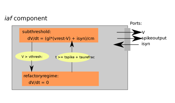
The corresponding code to generate this component is:
r1 = al.Regime(name = "subthresholdregime",
    time_derivatives = ["dV/dt = ( gl*( vrest - V ) + ISyn)/(cm)"],
    transitions = [al.On("V > vthresh",
                         do=["tspike = t",
                             "V = vreset",
                             al.OutputEvent('spikeoutput')],
                         to="refractoryregime")])
r2 = al.Regime(name="refractoryregime",
               time_derivatives=["dV/dt = 0"],
iaf = al.Dynamics(
    name = "iaf",
    dynamics = al.Dynamics( regimes = [r1,r2] ),
    analog_ports=[al.SendPort("V"), al.ReducePort("ISyn", reduce_op="+")],
    event_ports=[al.SendEventPort('spikeoutput')])
Similarly, we can define a synapse component:
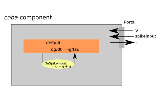
with corresponding code:
coba = al.Dynamics(
     name = "CobaSyn",
     dynamics =
        al.Dynamics(
            aliases = ["I:=g*(vrev-V)", ],
            regimes = [
              al.Regime(
                 name = "cobadefaultregime",
                 time_derivatives = ["dg/dt = -g/tau",],
                 transitions = [
                     al.On(al.InputEvent('spikeinput'), do=["g=g+q"]),
                     ],
                 )
                ],
            state_variables = [ al.StateVariable('g') ]
            ),

     analog_ports = [ al.RecvPort("V"), al.SendPort("I"), ],
     event_ports = [al.RecvEventPort('spikeinput') ],
     parameters = [ al.Parameter(p) for p in ['tau','q','vrev']  ]
     )
Multi-Dynamics
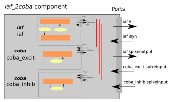
We now define a larger component, which will contain these sub_dynamics. When we create the component, we specify the name of each subcomponent, which allows us to reference them in the future.
We also need to specify that the voltage send port from the iaf needs to be connected to the voltage receive ports of the synapse. Similarly we need to connect the current port from the synapses into the current reduce port on the IAF neuron. These connections are shown in red on the diagram, and correspond to the arguments corresponding to the port_connections argument.
In a diagram:
In code:
# Create a model, composed of an iaf neuron, and
iaf_2coba_comp = al.MultiDynamics(name="iaf_2coba",
                                  sub_dynamics={"iaf" : get_iaf(),
                                                "coba_excit" : get_coba(),
                                                "coba_inhib" : get_coba()},
                                  port_connections=[
                                      ("iaf", "V", "coba_excit", "V"),
                                      ("iaf", "V", "coba_inhib", "V"),
                                      ("coba_excit", "I", "iaf", "ISyn"),
                                      ("coba_inhib", "I", "iaf", "ISyn")]